VBphenoR: Patient Phenotyping from Electronic Health Records using Variational Bayes

Brian Buckley, Adrian O’Hagan, Marie Galligan

This is the vignette for package VBphenoR.

Introduction

We previously implemented a patient phenotyping LCA model, Buckley et al. (2024) [1], using automatic differentiation variational inference (ADVI) available in the Stan [2] and PyMC3 [3] software . Although this approach delivered reasonable results, it required significantly complex technical tuning and multiple trial-and-error iterations. We find automatic VB methods as implemented in Stan VB are complex to configure and are very sensitive to model definition and algorithm hyperparameters such as choice of gradient optimiser.

In this R package [4] we now propose a closed-form approach based on the theory defined in Bishop (2006) [5], Nakajima et al. (2019) [6] and the review of Blei et al. (2017) [7]. We implement a variational Bayes Gaussian Mixture Model (GMM) algorithm using the closed-form coordinate ascent variational inference (CAVI) approach to determine the phenotype latent class, then implement a variational Bayes logit regression based on Durante & Rigon (2019) [8], where we determine the probability of the phenotype in the supplied cohort, the shift in biomarkers for patients with the phenotype of interest versus a normal population along with sensitivity analysis of binary indicator clicical codes and medication codes. The logit model likelihood uses the latent class from the GMM step to inform the conditional (see section 2.2 in [1]).

The implementation of VBphenoR performs the following steps:

1. Run a variational Gaussian Mixture Model using EHR-derived patient characteristics to discover the latent variable \(D_i\) indicating the phenotype of interest for the \(i^{th}\) patient. Patient characteristics can be any patient variables typically found in EHR data e.g.

   • Gender
   • Age
   • Ethnicity (for disease conditions with ethnicity-related increased risk)
   • Physical e.g. BMI for Type 2 Diabetes
   • Clinical codes (diagnosis, observations, specialist visits, etc.)
   • Prescription medications related to the disease condition
   • Biomarkers (usually by laboratory tests)

2. Run a variational Regression model using the latent variable \(D_i\) derived in step 1 as an interaction effect to determine the shift in biomarker levels from baseline for patients with the phenotype versus those without. Appropriately informative priors are used to set the biomarker baseline.

3. Run a variational Regression model using the latent variable derived in step 1 as an interaction effect to determine the sensitivity and specificity of binary indicators for clinical codes, medications and availability of biomarkers (since biomarker laboratory tests will include a level of missingness).

In the following example we use the Sickle Cell Disease (SCD) data available in this package to find the rare phenotype. SCD is extremely rare so we use DBSCAN to initialise the VB GMM. We also use an informative prior for the mixing coefficient and stop iterations when the ELBO starts to reverse so that we stop when the minor (SCD) component is reached.

\(\\\)

library(data.table)

# Load the SCD example data supplied with the VBphenoR package
data(scd_cohort)

# We will use the SCD biomarkers to discover the SCD latent class
X1 <- scd_cohort[,.(CBC,RC)]
 
# We need to supply DBSCAN hyper-parameters as we will initialise VBphenoR
# with DBSCAN. See help(DBSCAN) for details of these parameters.
initParams <- c(0.15, 5)
names(initParams) <- c('eps','minPts')

# X1 is the data matrix for the VB GMM
X1 <- t(X1) 

# Set an informative prior for the VB GMM mixing coefficient alpha 
# hyper-parameter
prior_gmm <- list(
  alpha = 0.001
)

# Set informative priors for the beta coefficients of the VB logit
prior_logit <- list(mu=c(1,
                   mean(scd_cohort$age),
                   mean(scd_cohort$highrisk),
                   mean(scd_cohort$CBC),
                   mean(scd_cohort$RC)),
              Sigma=diag(1,5))           # Simplest isotropic case

# X2 is the design matrix for the VB logit
X2 <- scd_cohort[,.(age,highrisk,CBC,RC)] 
X2[,age:=as.numeric(age)]
X2[,highrisk:=as.numeric(highrisk)]
X2[,Intercept:=1]
setcolorder(X2, c("Intercept","age","highrisk","CBC","RC"))

set.seed(123)
pheno_result <- runModel(scd_cohort,
                        gmm_X=X1, gmm_k=k, gmm_init="DBSCAN",
                        gmm_initParams=initParams,
                        gmm_maxiters=20, gmm_prior=prior_gmm,
                        gmm_stopIfELBOReverse=TRUE,
                        logit_X=X2, logit_prior=prior_logit
)

# Biomarker shifts for phenotype of interest
pheno_result$biomarker_shift

#   CBC_shift RC_shift
# 1      7.93     3.67

Details

Variational Gaussian Mixture Model

We employ a variational Gaussian Mixture Model (GMM) to detect the latent class for patients with the disease condition based on patient characteristics. The full derivation for the GMM can be found in Bishop (2006) [5]. Here, we explain how the posterior is affected by informative priors. The derivation in Bishop (2006) uses conjugate priors to simplify the analysis so we implement the same conjugacy in this package.

The conjugate prior for the GMM mixing coefficients, \(\pi\), is a Dirichlet distribution with prior hyperparameter \(\alpha\).

\[q(\bf{\pi}) = \textit{Dir}( \bf{\pi}|\alpha)\] The conjugate prior governing the unknown mean and precision of each GMM multivariate Gaussian component is an independent Gaussian-Wishart prior.

\[q(\bf{\mu}, \bf{\Lambda}) = \mathbb{N}(\bf{\mu}|\bf{m}, (\beta\bf{\Lambda})^{-1})\mathbb{W}(\bf{\Lambda}|\bf{W}, \nu)\]

Where

• \(\beta\) governs the proportionality of the precision, \(\Lambda\)
• \(W\) is a symmetric, positive definite matrix with dimensions given by the number of mixture components and governs the unknown precision of each GMM multivariate Gaussian component
• \(m\) is a prior hyperparameter governing the mean vector for the normal part. This is usually defaulted to the row means of the data. A different value can be used in rare cases where there is some specific prior clinical evidence that the cluster means should fall in a specific region away from the data mean.
• \(\nu\), the degrees of freedom, ensures the Wishart \(\Gamma\) function is well-defined. \(\nu\) must be greater than \(D-1\) (where \(D\) is the dimensionality of the data) to ensure the distribution is proper and the mean of the Wishart (\(\nu W^{-1}\)) exists. This is usually defaulted to \(D+1\) as it is the smallest value that ensures the Wishart distribution is proper and the expected value of the precision matrix exists. This value also results in a vague prior. It could be increased if there is a desire to avoid overly flexible or noisy covariance estimates.

Effect of informative priors

Informative priors play an important role in the variational model. In this section we will briefly outline the prior effects on the VB posterior estimates. For a full explanation please see [5]. We use the kmeans “init” option for the illustration as the faithful data is simple. For complex data, such as our Sickle Cell Disease data, where the disease-positive class is extremely unbalanced (0.3%) and covered by a very noisy tail from the negative class, we use DBSCAN instead.

Prior hyperparameter \(\alpha\) for the mixing Dirichlet distribution.

The prior for the GMM mixing coefficients, \(\pi\), affects the expectation such that if \(\alpha \longrightarrow 0\), then the posterior distribution will be influenced primarily by the data and as \(\alpha \longrightarrow \inf\) then the prior will have increased influence on the posterior.

To illustrate in Figure 1, we use the base R faithful data with three different values for \(\alpha\) (low, medium and high) and set \(k=6\). In this simplest case, we use the same \(\alpha\) value for each component. As alpha increases, the number of cluster components clearly approaches the desired k. However, a lower alpha tends to produce a more intuitive number of components for these data. In a realistic clinical setting, prior clinical knowledge can be used to guide the selection of alpha, allowing us to balance the number of components in a way that provides meaningful clinical insight while minimising the risk of bias introduced by setting alpha too high.

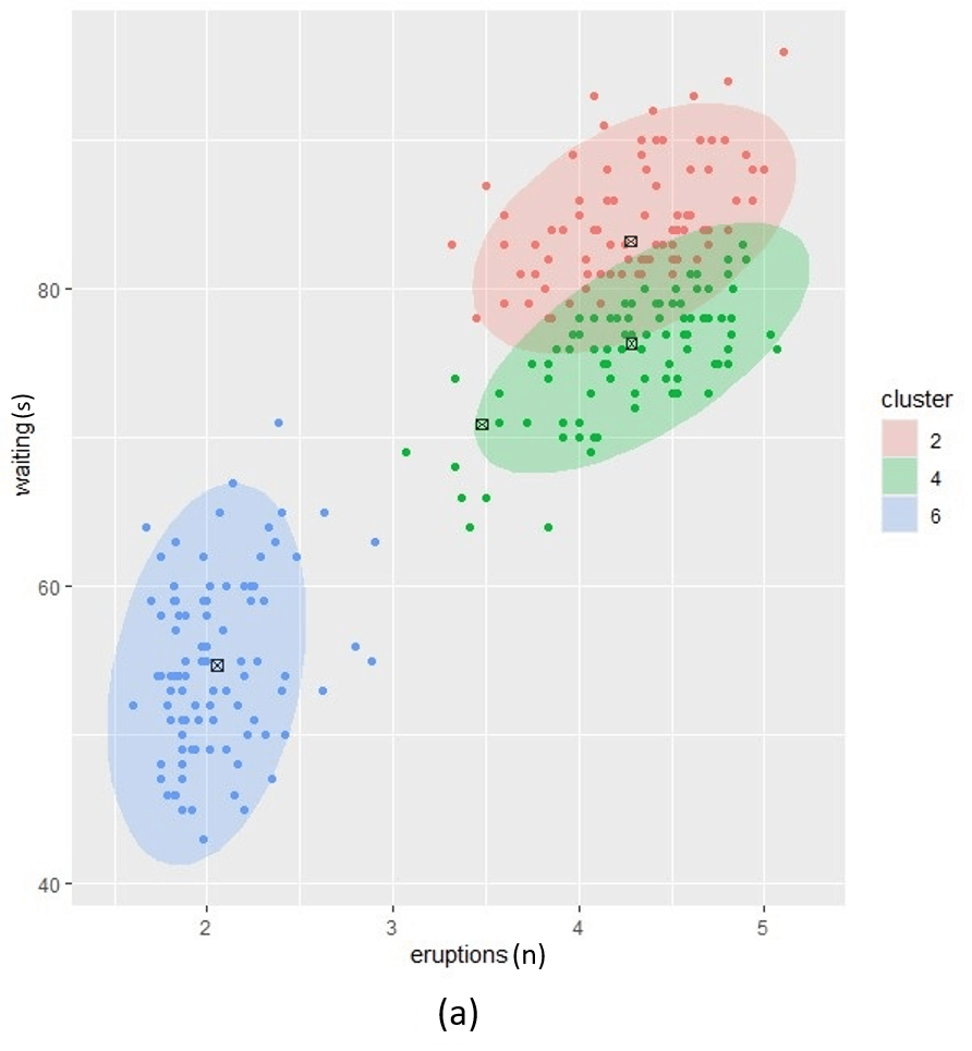
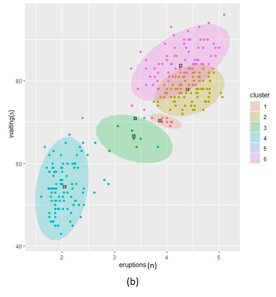
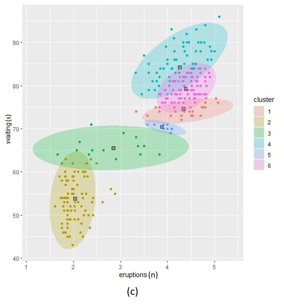
Figure1. Posterior clustering with three alpha prior hyperparameter settings. (a); low alpha setting, (c); high alpha setting and (b); a setting between low and high.

If we use different \(\alpha\) values for each cluster we can further fine-tune the resulting posterior. In Figure 2, we illustrate three different settings where the \(\alpha\) per cluster is equal and set low (left), equal and set high (right) and different per cluster component (middle). In this example we set \(k=4\).

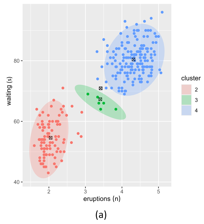
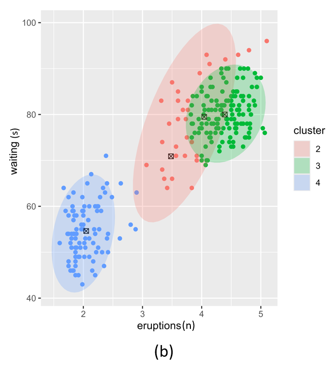
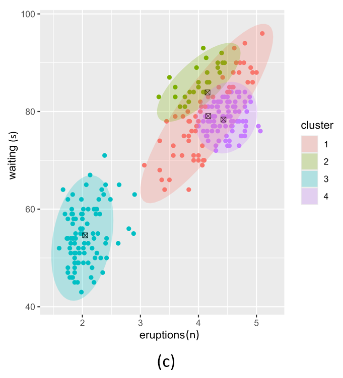
Figure 2. Posterior clustering with three different alpha vector prior hyperparameter settings. (a); equal alpha vectors, (c); different alpha vectors and (b); two equal and two different alpha vectors.

\(\\\)

Prior hyperparameter \(\beta\) for pseudo-observations for the Gaussian-inverse Wishart distribution.

The \(\beta\) prior has a significant effect on the posterior as shown in Figure 3. Here, we show the effect of a very low value for \(\beta\) and a very high value for \(\beta\). Low values for \(\beta\) lead to weaker distributions around \(m\). In this case the posterior means, \(\mu_k\), will be driven mainly by the data assigned to each cluster. On the contrary, high \(\beta\) values encode a strong belief that component means are close to \(m\).

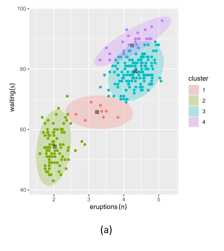
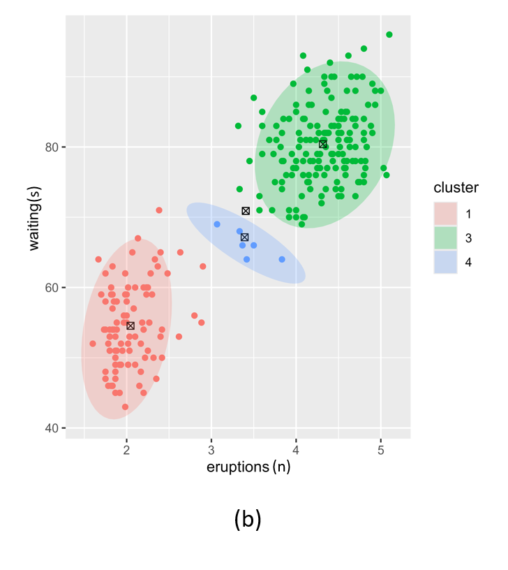
Figure 3. Posterior clustering with two different beta vector prior hyperparameter settings. (a); low beta vectors, (b); high beta vectors.

\(\\\)

Prior hyperparameter \(W\) for the scale matrix for the inverse Wishart.

The \(W\) prior for the Normal-Wishart posterior also has a significant effect on the posterior as illustrated in Figure 4. Low values for \(W\) results in more clusters that are likely to be more compact. This risks overfitting. Higher values of \(W\) result in broad, low-precision Gaussians. This risks underfitting.

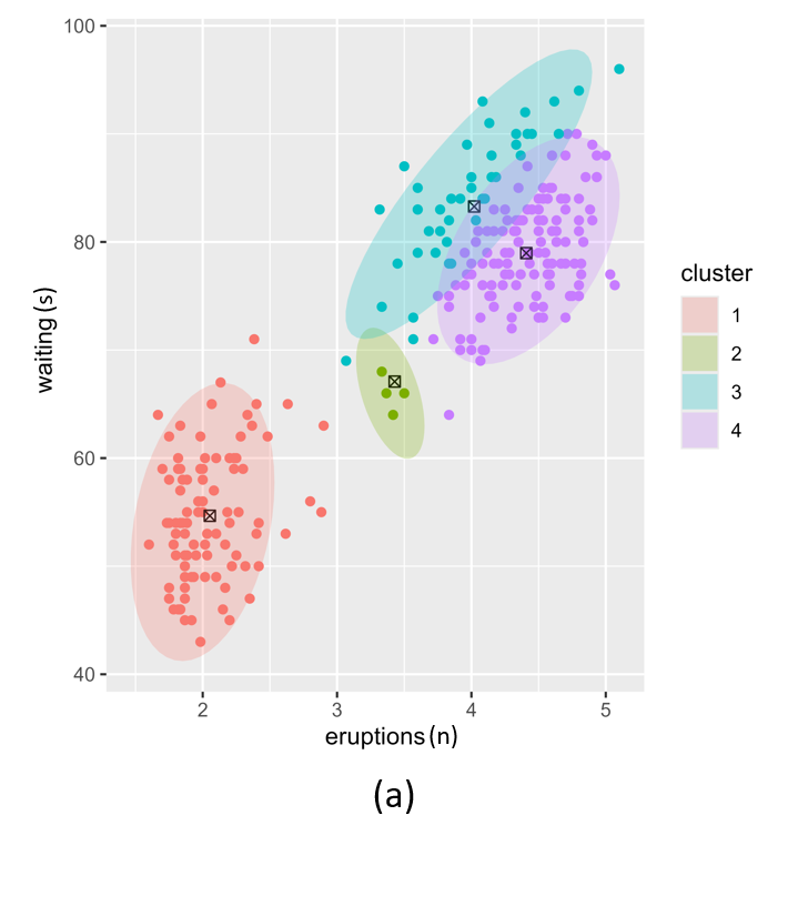
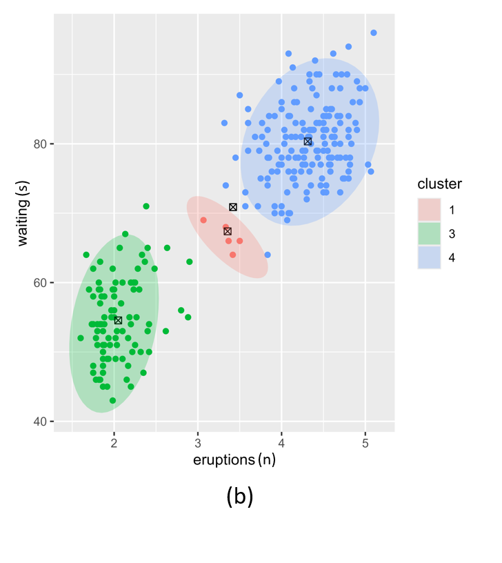
Figure 4. Posterior clustering with two different W vector prior hyperparameter settings. (a); low W vectors, (b); high W vectors.

\(\\\)

The following examples were used to generate Figures 2, 3 and 4.

  data("faithful")
  X <- faithful
  P <- ncol(X)

  # Run with 4 presumed components for demonstration purposes
  k = 4

  # ------------------------------------------------------------------------------
  # Plotting
  # ------------------------------------------------------------------------------

  #' Plots the GMM components with centroids
  #'
  #' @param i List index to place the plot
  #' @param gmm_result Results from the VB GMM run
  #' @param var_name Variable to hold the GMM hyperparameter name
  #' @param grid Grid element used in the plot file name
  #' @param fig_path Path to the directory where the plots should be stored
  #'
  #' @returns
  #' @importFrom ggplot2 ggplot
  #' @export

  do_plots <- function(i, gmm_result, var_name, grid, fig_path) {
    dd <- as.data.frame(cbind(X, cluster = gmm_result$z_post))
    dd$cluster <- as.factor(dd$cluster)

    # The group means
    # ---------------------------------------------------------------------------
    mu <- as.data.frame( t(gmm_result$q_post$m) )

    # Plot the posterior mixture groups
    # ---------------------------------------------------------------------------
    cols <- c("#1170AA", "#55AD89", "#EF6F6A", "#D3A333", "#5FEFE8", "#11F444")
    p <- ggplot() +
      geom_point(dd, mapping=aes(x=eruptions, y=waiting, color=cluster)) +
      scale_color_discrete(cols, guide = 'none') +
      geom_point(mu, mapping=aes(x = eruptions, y = waiting), color="black",
                 pch=7, size=2) +
      stat_ellipse(dd, geom="polygon",
                   mapping=aes(x=eruptions, y=waiting, fill=cluster),
                   alpha=0.25)

    plots[[i]] <- p
    rm(gmm_result, dd, mu)
    gc()

    grids <- paste((grid[i,]), collapse = "_")
    ggsave(filename=paste0(var_name,"_",grids,".png"), plot=p, path=fig_path,
           width=12, height=12, units="cm", dpi=600, create.dir = TRUE)
  }

  # ------------------------------------------------------------------------------
  # Dirichlet alpha
  # ------------------------------------------------------------------------------
  alpha_grid <- data.frame(c1=c(1,1,183),
                           c2=c(1,92,92),
                           c3=c(1,183,198),
                           c4=c(1,198,50))
  init <- "kmeans"

  z <- vector(mode="list", length=nrow(alpha_grid))
  plots <- vector(mode="list", length=nrow(alpha_grid))

  # Just plot the first 5 grids to save time
  for (i in 1:nrow(alpha_grid)) {
    prior <- list(
      alpha = as.integer(alpha_grid[i,]) # set most of the weight on one component
    )

    gmm_result <- vb_gmm_cavi(X=X, k=k, prior=prior, delta=1e-9, init=init,
                              verbose=FALSE, logDiagnostics=FALSE)
    z[[i]] <- table(gmm_result$z_post)
    do_plots(i, gmm_result, "alpha", alpha_grid, gen_path)
  }

  # ------------------------------------------------------------------------------
  # Normal-Wishart beta for precision proportionality
  # ------------------------------------------------------------------------------
  beta_grid <- data.frame(c1=c(0.1,0.9),
                          c2=c(0.1,0.9),
                          c3=c(0.1,0.9),
                          c4=c(0.1,0.9))
  init <- "kmeans"

  z <- vector(mode="list", length=nrow(beta_grid))
  plots <- vector(mode="list", length=nrow(beta_grid))

  # Just plot the first 5 grids to save time
  for (i in 1:nrow(beta_grid)) {
    prior <- list(
      beta = as.numeric(beta_grid[i,])
    )

    gmm_result <- vb_gmm_cavi(X=X, k=k, prior=prior, delta=1e-9, init=init,
                              verbose=FALSE, logDiagnostics=FALSE)
    z[[i]] <- table(gmm_result$z_post)
    do_plots(i, gmm_result, "beta", beta_grid, gen_path)
  }

  # ------------------------------------------------------------------------------
  # Normal-Wishart W0 (assuming variance matrix) & logW
  # ------------------------------------------------------------------------------

  w_grid <- data.frame(w1=c(0.001,2.001),
                       w2=c(0.001,2.001))
  init <- "kmeans"

  z <- vector(mode="list", length=nrow(w_grid))
  plots <- vector(mode="list", length=nrow(w_grid))

  # Just plot the first 5 grids to save time
  for (i in 1:nrow(w_grid)) {
    w0 = diag(w_grid[i,],P)
    prior <- list(
      W = w0,
      logW = -2*sum(log(diag(chol(w0))))
    )

    gmm_result <- vb_gmm_cavi(X=X, k=k, prior=prior, delta=1e-9, init=init,
                              verbose=FALSE, logDiagnostics=FALSE)
    z[[i]] <- table(gmm_result$z_post)
    do_plots(i, gmm_result, "w", w_grid, gen_path)
  }

Effect of initialiser

The VB GMM can be initialised using one of four methods:

1. kmeans
2. DBSCAN
3. Random assignment

kmeans is the default as it is simple, computationally fast and gives reasonable estimates if the data are not too complex In cases of complex data, such as the Sickle Cell Disease sample data included in the package, we recommend DBSCAN. The Random assignment option is rarely useful but is included for completeness. If there are more components in the result than you require we recommend HDBSCAN to merge unwanted clusters. \(\\\)

VB GMM example using kmeans

Figure 5 illustrates the challenges when using kmeans as an initialiser for an extremely unbalanced data set, e.g. the scd_cohort data included in this package. kmeans is a good option where data is not overly unbalanced as it is very computationally fast. But it is unable to cope with very noisy and highly unbalanced cluster classes.

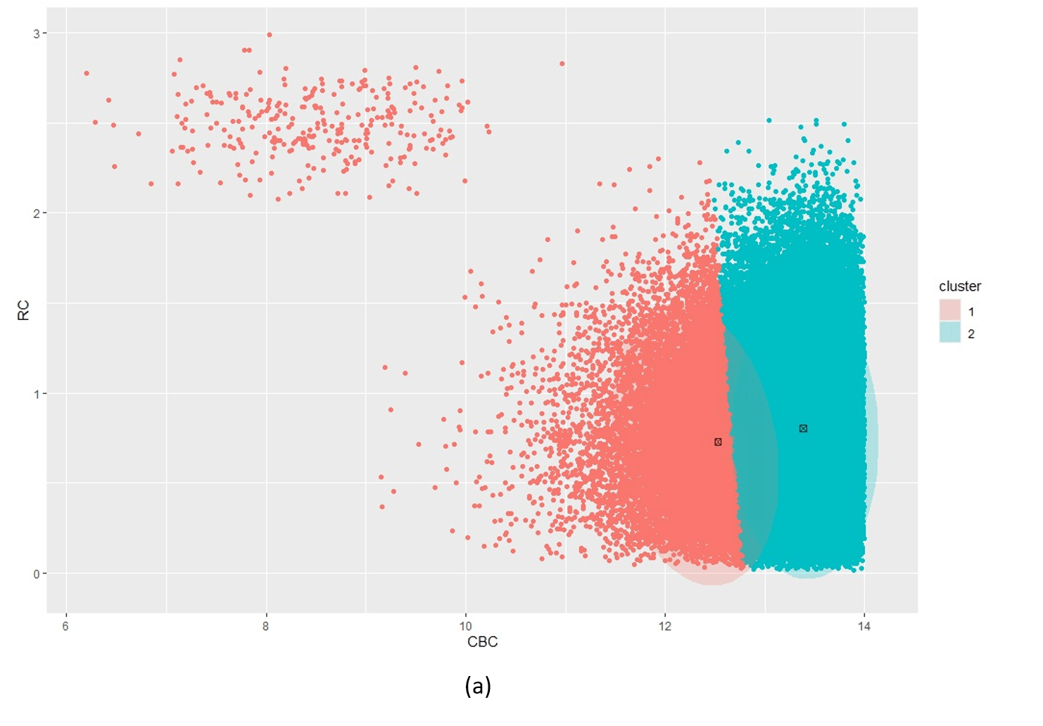
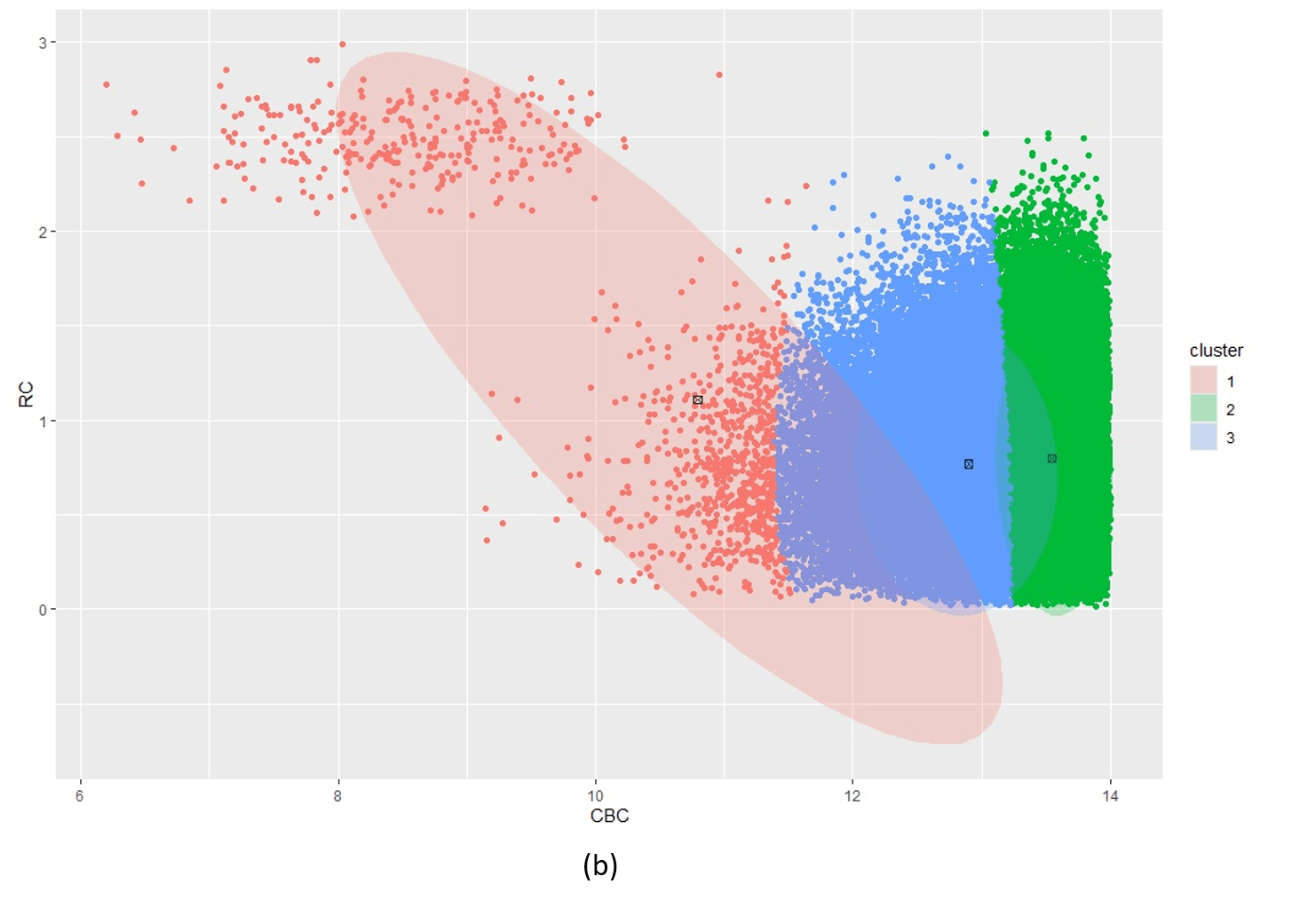
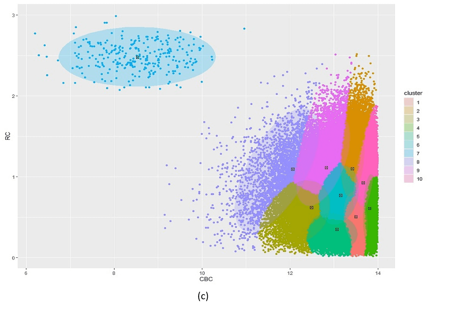
Figure 5: Posterior clustering of SCD Cohort using kmeans as initialiser. With k=2 (a) the model cannot distinguish the rare SCD cluster from the majority class. With k=3 (b), the model is starting to find the SCD cluster but there is still too much overlap so the cluster centroid is far from the true SCD cluster. We have to go all the way to k=10 (c) before the SCD cluster is identified.

\(\\\)

VB GMM example using DBSCAN

Figure 6 is a single run using DBSCAN as the initialiser for the highly unbalanced and noisy scd_cohort data. DBSCAN is very capable of finding the rare phenotype class and thus provides excellent starting positions for the VB GMM. This is at the cost of computational performance. While kmeans runs in less than a second, DBSCAN takes about 16 seconds for these data. Another issue with DBSCAN is that it cannot be limited to a specified number of clusters so it often returns more than k clusters when k is small e.g. k = 2 in our current phenotyping model. We therefore need to merge clusters returned by DBSCAN before passing the correct number k cluster centroids to VB GMM.

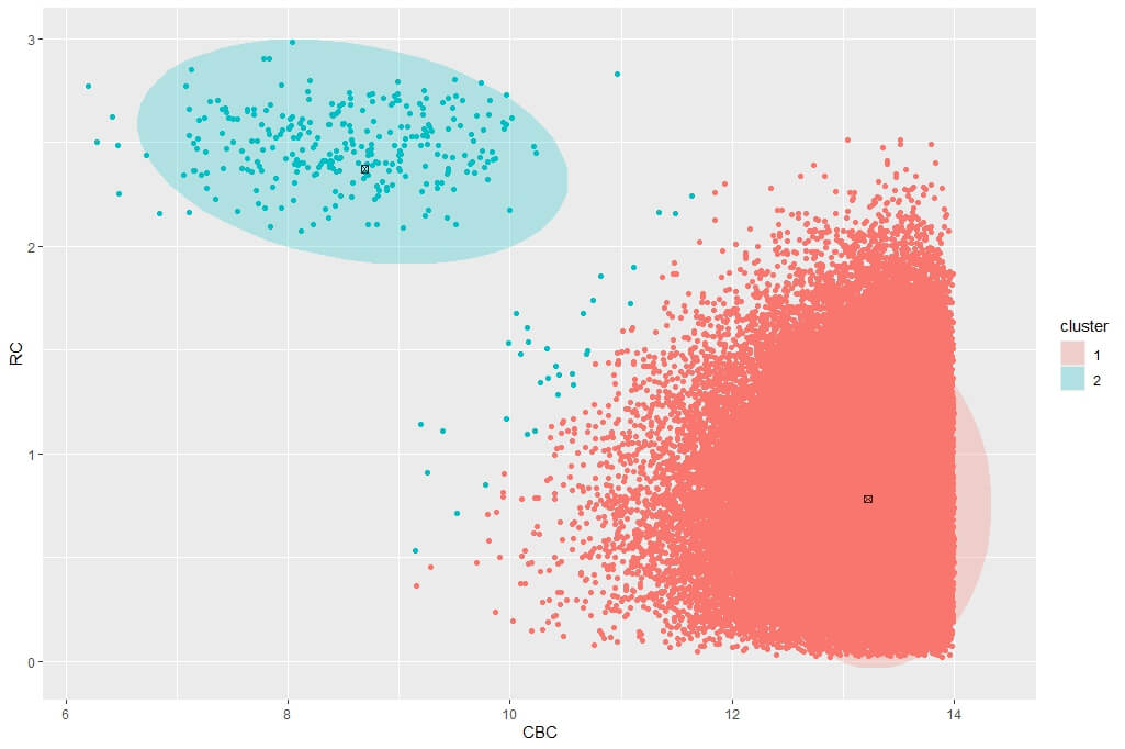
Figure 6: Posterior clustering of SCD Cohort using DBSCAN as initialiser using k=2. The SCD cluster is found by the model, albeit with some misclassified non-SCD observations on the boundary with the majority class.

Example R code to run all examples above can be found in the manual page for vb_gmm_cavi and VBphenoR.

Variational Logit

We employ a variational logit regression to classify the patients with the disease condition, given the latent class we obtained from the VB GMM. In canonical logistic regression, the response variable \(y_i\) is binary and the likelihood for \(y_i\) is

\[ P(y_i|X_i,\beta) = \sigma(X^T_i\beta)^{y_i} \cdot [1 - \sigma(X^T_i\beta)]^{1-y_i}\] where:

• \(X_i\) is the feature vector for observation \(i\),
• \(\beta\) is the vector of coefficients,
• \(\sigma(z) = \frac{1}{1 + e^{-z}}\) is the logistic i.e. sigmoid function.

Effect of informative priors

To perform Bayesian Inference, we specify a prior distribution for the coefficients \(\beta\). A common choice is a multivariate normal prior for the true posterior:

\[P(\beta) = \mathbb{N}(\beta|m_0, S_0)\] where:

• \(m_0\) is the prior mean vector assumption for the true (unknown) mean vector,
• \(S_0\) is the prior coveriance matrix for the true (unknown) covariance matrix.

In variational Inference, the prior is part of the Kullback-Leibler divergence [7] between the approximate posterior \(Q(\beta)\) and the true posterior \(P(\beta)\):

\[KL(Q(\beta) || P(\beta))\] where:

\[Q(\beta) = \mathbb{N}(\beta|m,S)\] and,

• \(m\) is the best-fit approximate mean vector,
• \(S\) is the best-fit approximate covariance matrix

This effect is used for optimising the variational parameters by maximising the Evidence Lower Bound (ELBO) [7], which is a lower bound on the log marginal likelihood:

\[ELBO = \mathbb{E}_{Q(\beta)}[log P(y|X,\beta)] - KL(Q(\beta)||P(\beta))\] If we use uninformative priors for \(m_0\) and \(S_0\), we reduce the model to essentially maximum likelihood given the data. In clinical settings, we usually have expert medical opinion or empirical evidence that can be used to set informative priors. This approach can enhance the clinical value of the posterior results and overcome some of the limitations in EHR data, such as missing biomarker data and high levels of imbalance in the response. \(\\\)\(\\\)

References

[1]

Buckley, B., O’Hagan, A. and Galligan, M. (2024). Variational Bayes latent class analysis for EHR-based phenotyping with large real-world data. Frontiers in Applied Mathematics and Statistics 10 1302825.

[2]

Carpenter, B., Gelman, A., Hoffman, M. D., Lee, D., Goodrich, B., Betancourt, M., Brubaker, M., Guo, J., Li, P. and Riddell, A. (2017). Stan: A probabilistic programming language. Journal of Statistical Software 76.

[3]

Salvatier, J., Wiecki, T. V. and Fonnesbeck, C. (2016). Probabilistic programming in Python using PyMC3. PeerJ Computer Science 2 p55.

[4]

Grunsky, E. (2002). R: A data analysis and statistical programming environment–an emerging tool for the geosciences. Computers & Geosciences 28 1219–22.

[5]

Bishop, C. M. and Nasrabadi, N. M. (2006). Pattern Recognition and Machine Learning. vol 4 Springer.

[6]

Nakajima, S., Watanabe, K. and Sugiyama, M. (2019). Variational Bayesian Learning Theory. Cambridge University Press.

[7]

Blei, D. M., Kucukelbir, A. and McAuliffe, J. D. (2017). Variational inference: A review for statisticians. Journal of the American statistical Association 112 859–77.

[8]

Durante, D. and Rigon, T. (2019). Conditionally conjugate mean-field variational Bayes for logistic models. Statistical Science 34 472–85.